Calculating Aerodynamic Forces and Moments

The most accurate forces and moments are normally those output by your flow solver, which knows details of your solution’s boundary conditions and can use modeling such as turbulent wall functions that Tecplot cannot. If your solver’s calculations are not available, you can use Tecplot’s Analyze/Perform Integration… option with the Forces and Moments integration type. There are cases where you want more control over the calculation, however, so this document details additional methods by which you may calculate these quantities. For any of these calculations, it is necessary to be able to calculate usable surface normal vectors, so we’ll discuss those first.

Surface Normal Vectors for FE (Unstructured) Surface Zones

For finite-element (triangular/quadrilateral) surface zones, Tecplot uses the node ordering of each cell with the right-hand rule to determine that cell’s unit normal. For the resultant forces and moments to be correct with any of the methods presented here, including Tecplot’s Forces and Moments integration, these normals must be consistent—they must all point away from one side or the other of the surface. Further, if the normals point into the body instead of into the fluid, the signs of the calculated forces and moments will be reversed. You can check your data set by the following procedure:

Select Analyze/Calculate Variables… to calculate Grid K Unit Normal; choose Cell Center for New Var Location.
Select Plot/Vector/Variables to choose X Grid K Unit Normal, Y Grid K Unit Normal, and Z Grid K Unit Normal as the vector variables.
Click Zone Style… in Tecplot’s sidebar, click the Points tab, select your surface zones, right-click under Points to Plot, and select Surface cell centers.
Click the Vector tab and ensure Show Zone and Show Vector are checked for each surface zone.
Toggle on the Vector layer in Tecplot’s sidebar.
If you cannot see the vectors, or if they are too long, adjust their length by choosing Plot/Vector/Details…
Ensure vectors all point out of the same side of your surface. If the vectors point into the body instead of into the fluid, remember to negate the forces and moments you calculate.

Now we’ll cover three scenarios: Pressure-only calculation on surfaces, pressure and supplied shear stress on surfaces, and calculation when surface shear stress is not available but the volume velocity field is available.

From Pressure Only on Surfaces.

If you are interested only in the contributions of pressure—your flow is inviscid, for example—you may calculate forces and moments on surface zones by the following procedure:

Select Analyze/Calculate Variables… to calculate Grid K Unit Normal; choose Cell Center for New Var Location.
Select Data/Alter/Specify Equations… with the following equations; specify Cell Center for New var location:
{px} = -{Pressure} * {X Grid K Unit Normal} {py} = -{Pressure} * {Y Grid K Unit Normal} {pz} = -{Pressure} * {Z Grid K Unit Normal} {mx} = Y * {pz} – Z * {py} {my} = Z * {px} – X * {pz} {mz} = X * {py} – Y * {px}
Select Analyze/Perform integration to perform a scalar Integration of each of the last 6 items to calculate, respectively, X-, Y- and Z-Force, and X-, Y- and Z-Moment.

From Pressure and Supplied Shear Stress on Surfaces

If your flow is viscous and your data set includes viscous shear stress for your surface zones, you can modify step 2 above to include the effects of viscosity. If, for example, your data set includes variables named tx, ty and tz representing the viscous shear stress, then calculate Grid K Unit Normal as above, but modify step 2 to use the following equations:
{taux} = {tx} – {X Grid K Unit Normal} * {Pressure} {tauy} = {ty} – {Y Grid K Unit Normal} * {Pressure} {tauz} = {tz} – {Z Grid K Unit Normal} * {Pressure} {mx} = Y * {tauz} – Z * {tauy} {my} = Z * {taux} – X * {tauz} {mz} = X * {tauy} – Y * {taux}
Integrate each of these 6 variables over your surface(s) to calculate forces and moments.

From Pressure and Velocity Field

If your flow is viscous but your surface zones do not include surface shear stress variables, the velocity gradient on the surface zones must be calculated from your solution’s volume velocity field. This requires you to load both the surface zones on which you wish to calculate the forces and moments, and volume zones that provide the velocity field next to these surfaces.

The below calculations rely on Tecplot’s velocity gradient calculation. When using ordered (structured) grids, these are done using standard curvilinear coordinate transformations. Using finite-element (unstructured) grids, these are done using a moving least-squares technique. For more details of these calculations, please refer to User’s Manual.

To allow you to modify the following procedure to suit the specifics of your data, we’ll cover the involved equations in detail. If we accept Stokes’ hypothesis that the second coefficient of viscosity is zero (see for example https://assets.press.princeton.edu/chapters/s10157.pdf), then the Newtonian stress tensor is:

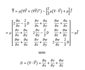
µ is the dynamic viscosity, p is pressure, and I is the identity matrix. The stress on a surface is equal to the stress tensor dotted with the surface unit normal (which must point away from the surface—into the fluid flow):
The above can be simplified for 2D by removing any equations with w or z (or setting w=0 and d/dz = 0). Integrating each of the resulting vector components gives the components of the force the fluid is exerting on the surface. We can also calculate the moment due to fluid stress by taking the vector cross product of the displacement vector (from the origin) and the stress vector:

Integrating each of the resulting components produces the X-, Y- and Z-moments about the chosen origin.

Calculating in Tecplot 360

To perform all of this in Tecplot, ensure that you have both volume zones containing the fluid velocity and surface zones that represent the surfaces on which you wish to calculate forces and moments. Then perform the following steps:

Select Analyze/Calculate Variables… to calculate Velocity Gradient (nodal, not calculate-on-demand).
Select Data/Interpolate/Linear to interpolate the components of the velocity gradient (dUdX, dVdX,…,dWdZ) from volume zones to surface zone(s) of interest.
Select Analyze/Calculate Variables… to calculate Grid K Unit Normal (cell-centered).
Select Data/Alter/Specify Equations with the following equations, replacing <mu> with the dynamic viscosity of your fluid (consistent with the dimensions or nondimensionalization of your data); specify Cell Center for New var location:
{D} = {dUdX} + {dVdY} + {dWdZ} {T11} = <mu> * (2 * {dUdX} - 2/3 * {D}) - {Pressure} {T12} = <mu> * ({dVdX} + {dUdY}) {T13} = <mu> * ({dWdX} + {dUdZ}) {T22} = <mu> * (2 * {dVdY} - 2/3 * {D})-{Pressure} {T23} = <mu> * ({dVdZ} + {dWdY}) {T33} = <mu> * (2 * {dWdZ} - 2/3 * {D}) - {Pressure} {taux} = {T11} * {X Grid K Unit Normal} + {T12} * {Y Grid K Unit Normal} + {T13} * {Z Grid K Unit Normal} {tauy} = {T12} * {X Grid K Unit Normal} + {T22} * {Y Grid K Unit Normal} + {T23} * {Z Grid K Unit Normal} {tauz} = {T13} * {X Grid K Unit Normal} + {T23} * {Y Grid K Unit Normal} + {T33} * {Z Grid K Unit Normal} {mx} = Y * {tauz} – Z * {tauy} {my} = Z * {taux} – X * {tauz} {mz} = X * {tauy} – Y * {taux}
Select Analyze/Perform integration… to perform a scalar Integration of each of the last 6 items over your surface zones to calculate, respectively, X-, Y- and Z-Force, and X-, Y- and Z-Moment.

Tecplot Knowledge Base