Creating Geometric Regions

A quick reference guide on how to create different geometric regions can be found at the bottom of this article.

In Tecplot 360, users may need to create a geometric region to perform operations such as extracting or blanking data. For example, an internal combustion engineer may want to quantify the temperature within a certain radius of a spark plug. By generating a sphere region around the spark plug and extracting that data, they are able to do so.

How is This Accomplished?

This can be achieved by generating new variables in Data>Alter>Specify Equations that represent each of a geometric shape’s system of equations. The generated variables can then be set equal to different values in Plot>Blanking>Value Blanking then extracted (if necessary, Data>Extract>Blanked Zones…) in order to generate a shape of certain parameters.

What Are the Limitations of This Method?

Some geometric shapes will require many equations to define them. For example, a simple plane can be generated with a single equation. For example:

{plane} = x + y + z

We can then generate a plane by generating an iso surface where {plane} equals 5.

5 = x + y + z

However, what if a user wants a plane with specific dimensions? For example, making our plane smaller so that it only appears within a 2x2x2 region. This will require 6 more constraints:

x<0;    x>2;    y<0;    y>2;    z<0;    z>2;

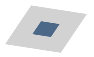
The grey section represents the plane before blanking constraints were applied. The blue represents the section now defined in our 2x2x2 region.

Each of these equations requires a unique blanking constraint in the Value Blanking dialog.

To work around this, users can define new variables in the Specify Equations dialog, then blank based on those new variables. For example, the six equations listed in the example above can be represented and blanked the same way by creating a new variable blank:

{blank} = IF(x<0 || x>2 || y<0 || y>2 || z<0 || z>2, 1, 0)

Then blank all values where blank equals 1:

While specifying a blanking variable can be a very powerful and flexible option, for larger data sets this method requires more computation to generate the variables across an entire data set compared to individual blanking constraints.

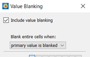
If a user wishes to blank halfway across a cell, but data only exists on the edges of the cell, blanking will not create a “clean cut” and slice the cell in half. Instead, Tecplot will only blank entire cells. To create a clean cut through the middle of cells, Tecplot would have to generate new data points along the intersection line, which would partially defeat the point of value blanking in the first place for most users.  The resolution of the blanking depends on the cell resolution.

This behavior can be adjusted slightly in the Plot>Blanking>Value Blanking dialog under the “Blank Entire Cell When:” option. This will allow a user to choose how cells are removed when intersected.

An Example Using a Cone Region

With eight blanking constraints, a user can generate cones, spheres, planes, and prisms using this method. A quick reference guide for each of these shapes can be found at the end of this article. The following detailed example will use a cone and some example data included with Tecplot360, located in the Examples>Simple Data folder inside the Tecplot360 installation folder. A cone will be constructed using an arctangent equation in the Specify Equations dialog.

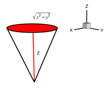
{cone} = atan2(sqrt(x**2 + y**2), z)

Load in Example Data and Prepare It

1. On your machine, navigate to the example data folder in the Tecplot installation directory and load in the example data plt. The following example is applicable to any 3D data, however, any specific equation translations or parameters in this example will be for the f18.plt data.
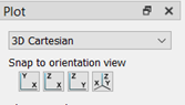
2. Select 3d Cartesian from the plot toolbar.
   
3. To better see our geometry later on in the example, we’ll create another zone to visualize it in. Inside Tecplot, navigate to Data>Create Zone>Rectangular and create a zone with these parameters:
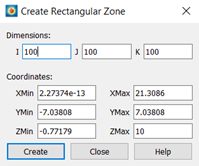   The only values changed from the defaults for this data are Dimensions I, J, K, and ZMax. It is not critical to get these dimensions exactly right. As mentioned above, these adjustments are only to create a larger, more detailed zone around the f18 data to see our geometric region more clearly.

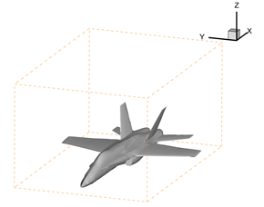
Final Product of “Load in Example Data and Prepare It”

Define the Variable Equations

Open the Specify Equations dialog under Data>Alter>Specify Equations and compute the following equation across all zones.

{cone}=atan2(sqrt((x-10)**2+y**2),(z+1))

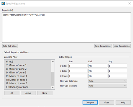
This {cone} variable has been set equal to a cone equation that was translated in order to align better with the f18.plt data. For a more general version of the cone equation with details on how user’s can translate their equations themselves, see the quick reference guide at the bottom of the article.

Here, two translations were made to the equation {cone} = atan2(sqrt(x**2 + y**2), z):

• x-10 : Moves the cone 10 units in the positive direction to be directly above the F18 airplane.
• Z+1 : Lowers the tip of the zone in the z direction by 1 unit, so that the cone extends through the entire F18 airplane.

Adjust Contour Settings to View the Geometric Region

Open the iso-surface and contour dialogs and adjust the mappings so that an enabled iso-surface will show the {cone} variable created in the previous step.

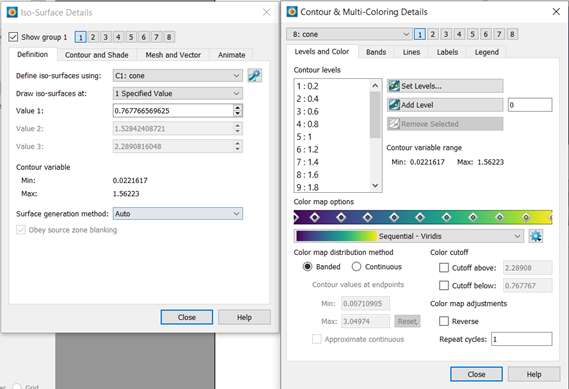
Make sure to set the iso-surface Value 1 to 0.5. Finally, enable iso-surfaces.

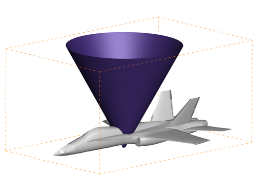
Final Product of “Adjust Value Blanking and Contour Settings to View the Geometric Region”

Blank and Extract Data

Navigate to Plot>Blanking>Value Blanking and blank any values “less than or equal to” 0.5. Remember, that 0.5 is only the outer most boundary of the cone. To remove all data inside the cone, you’ll need the “less than or equal to” option.

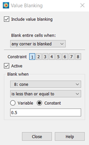
A hole in the F18 airplane data should appear where the cone was previously!

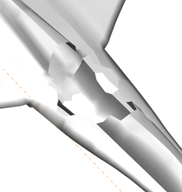
The hole created In “Blank and Extract Data”

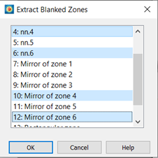
Finally, these blanked zones can be extracted. Navigate to Data>Extract>Blanked Zones. In this case, the following zones had a hole created in them and can be extracted:

nn4, nn.6, Mirror of nn.4, Mirror of nn.6

Tecplot 360 User’s Manual References

• Value Blanking
• Data Alter

Shapes

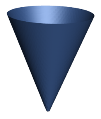Cone

{cone} = atan2(sqrt((x-x₀)**2 + (y-y₀)**2), (z-z₀))

• The sqrt() function generates a circular base plane for the cone. z represents the cone’s height from base to tip. These variables can be interchanged to rotate the axis of the cone.
• You can think of the iso-surface as the region on the plot where angle generated from the axis is equal to the arc tangent of (radius from the axis)/(axis distance from z0)
• x0, y0, and z0 represent position translation variables. For a cone generated at the origin, set these to zero.

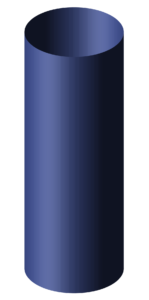
Cylinder

{cylinder_radius} = sqrt((x-x0)**2 + (y-y0)**2)

• (x0, y0) represents the center of the circular face of the cylinder.
• You can change the orientation of the cylinder’s axis by interchange x or y by z. In that case, (x0, z0) or (y0,z0) represent the circular cylinder face center.

Plane

{plane} = a(x-x₀) + b(y-y₀) + c(z-z₀)

• The plane will span the entire zone/dataset unless blanking constraints in Plot>Blanking>Value Blanking such as 0<x<2 are applied.
• x₀, y₀, and z₀ represent position translation variables. a, b, and c represent scalar translation variables.

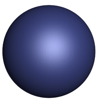Sphere

{sphere_radius} = sqrt((x-x0)**2 + (y-y0)**2 + (z-z0)**2)

(x0, y0, z0) represents the sphere’s origin point.

Rectangular Prism

A prism can be generated without an equation variable in Specify Equations. Rather, it can be created using only boundary constraints in Plot>Blanking>Value Blanking. For example, constraints for a 2x2x2 cube as shown:

x<0;    x>2;    y<0;    y>2;    z<0;    z>2;