


 MENU
MENUThis article describes both a macro and a PyTecplot script that extracts a field variable along a line normal to a surface. We recommend using PyTecplot insofar as possible.
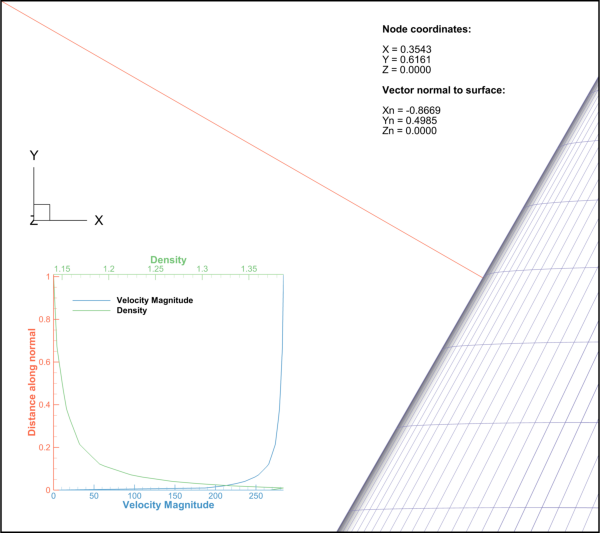
Figure 1: Velocity magnitude and Density VS distance along a line perpendicular to a surface
Example:
Load the M6-Wing example file, which can be found in your Tecplot Installation Directory:
…/Tecplot/Tecplot 360 EX 20xx R1/examples/OneraM6wing/OneraM6_SU2_RANS.plt.
To better visualize the node at which we’ll probe, let’s turn on the mesh for the second zone. Zoom somewhere on the wing and perform a probing while pressing Ctrl. This pins the probe to the nearest node.
Retrieve the zone number (2), and the node number in the Zone/Cell info tab in the probe sidebar. Launch the macro and enter the zone, node, and variable number as well as the extraction distance. We choose node 754 of zone 2, variable 4 (Density) and a distance of 1 in our example.
This node is located on the leading edge, around mid-span. See Figure 1.
PyTecplot
First, the script connects to an open instance of Tecplot. Make sure PyTecplot connections are enabled in the Scripting>PyTecplot Connections… menu and also include this in your script:
tp.session.connect()
The scripts then defines the point and surface from which the line is seeded, as well as the distance of extraction:
f=tp.active_frame()
p=tp.active_page()
ds=f.dataset
#define the surface zone, the node index and the distance to be extracted
zoneNr=2-1 #We use -1 because Tecplot indexes are 1-based, and PyTecplot is 0 based.
Zne=ds.zone(zoneNr)
nodeNr=754-1
distance=1
The vector normal to the surface is calculated calling an extended macro command:
#Calculation of the normal vector
tp.macro.execute_extended_command(command_processor_id='CFDAnalyzer4',
command=("Calculate Function='GRIDKUNITNORMAL' Normalization='None'"\
    +" ValueLocation='Nodal' CalculateOnDemand='F'"\
    +" UseMorePointsForFEGradientCalculations='F'"))
The variables names of the coordinates and surface normals are stored in lists:
#Identification of var names for coordinates and normal vector
coordVars=['x','y','z']
vectorVars=['X Grid K Unit Normal','Y Grid K Unit Normal','Z Grid K Unit Normal']
These lists can be called to compute the start point and end point of the line to be extracted:
#retrieves the start point(on the surface) and the end point of the line(offset)
surfPt=[Zne.values(i)[nodeNr] for i in coordVars]
endPt=[i+Zne.values(j)[nodeNr]*distance for i,j in zip(surfPt,vectorVars)]
The points along the line are stored in a numpy array:
#defines all of the points coordinates along the line:
linePts=np.zeros((3,100))
for i,(j,k) in enumerate(zip(surfPt,endPt)):
    linePts[i]=np.linspace(j, k, 100)
The line is then extracted:
#extract the line in Tecplot
line = tp.data.extract.extract_line(zip(linePts[0],linePts[1],linePts[2]))
Equations are used to compute the distance between each point and the surface:
#Compute the distance along the line
tp.data.operate.execute_equation(equation=\
    '{Dist}=SQRT(({'+'X}'+'-{}'.format(surfPt[0])+')**2'\
    +'+({'+'Y}'+'-{}'.format(surfPt[1])+')**2'\
    +'+({'+'Z}'+'-{}'.format(surfPt[2])+')**2)',
    zones=line)
Finally, the result is plotted in a new frame:
#Create a new frame for the plot
f2=p.add_frame()
f2.position=(4.3,5.0)
f2.height=3.2
f2.width=5.6
f2.plot_type=PlotType.XYLine
p=f2.plot()
p.delete_linemaps()
p.add_linemap()
p.linemap(0).name='Extracted Profile'
p.linemap(0).x_variable_index=3#default is the 4th variable
p.linemap(0).y_variable_index=ds.variable('Dist').index
p.linemap(0).zone_index=2
p.view.fit()
The 4th variable is plotted versus the distance to the surface, feel free to add a new fieldmap for each variable that is of interest.
Download ExtractBoundaryProfile.py from our handyscripts GitHub page.
Tecplot Macro:
The macro prompts the user for a node (on a surface-zone), a variable and a distance. A line is extracted at the surface normal of the node, with the entered distance. Finally, a XY Line plot of the user-given field variable VS the distance along the line is created.
The Extract Normal Profile macro is useful for the analysis of boundary layers, but also for determining ice-deposition on a surface.
Macro Commands:
The user is prompted via $!PROMPTFORTEXTSTRING commands to enter the variable, node, zone of interest and distance to extract the field variable:
$!PROMPTFORTEXTSTRING |nodenr|
  INSTRUCTIONS= "Node Number:"
These information can be retrieved by using the probing tool. To pin the probe to the nearest node, press Ctrl when performing the probe.
Then, the macro looks for an already existing distance variable using the $!GETVARNUMBYNAME command. If the variable exist, it will be deleted.
$!GETVARNUMBYNAME |vname|
  NAME = "dist"
$!IF "|vname|" == "dist"
  $!DELETEVARS  [|vname|]
$!ENDIF
The same reasoning is applied to the components of the vector normal to the surface. If at least one of the components doesn’t exist, the whole normal vector is being calculated.
The corresponding macro command can be found by recording the Analyze->Calculate Variable-> Grid K Unit Normal action in the GUI:
$!GETVARNUMBYNAME |xn|
  NAME = "X Grid K Unit Normal"
#idem for |yn| and |zn|
$!VARSET |varexists| = (|xn|*|yn|*|zn|)
$!IF |varexists| == 0
  $!EXTENDEDCOMMAND
    COMMANDPROCESSORID = 'CFDAnalyzer4'
    COMMAND = 'Calculate Function=\'GRIDKUNITNORMAL\'
               Normalization=\'None\' ValueLocation=\'Nodal\'
               CalculateOnDemand=\'F\'
               UseMorePointsForFEGradientCalculations=\'F\''
$!ENDIF
Then the $!GETVARNUMBYNAME commands are again called for xn, yn and zn; as we are yet sure they are calculated.
Yet the macro retrieves the (x,y,z) coordinates of the node on the surface, as well as the components of the normal vector at that point. All of this is achieved by calling the $!GETFIELDVALUE six times, with the appropriate zone, index and variable numbers.
The coordinates of the last point can be calculated by translating the surface point coordinates by the height times the normed-vector normal to the surface. Here a simple $!VARSET expression is used:
$!VARSET |xvecend| = (|xval|+|xnorm|*|height|)
#idem for yvecend and zvecend
A geometry is created between the surface point and the last point to be extracted. This is identical than the $!ATTACHGEOM command recorded from the Data->Extract->Extract Precise Line menu, with the following coordinates:
|xval|       |yval|       |zval|      #Point at the surface
|xvecend|    |yvecend|    |zvecend|   #Point at the end of the line
The geometry is extracted as a 100-points zone using the $!PICK command to select the geometry. The extraction is the performed over time (contrary to the Extract Precise Line macro), which means a 1D-100points zone will be created for each time step.
The extended macro command can be obtained by recording the Data->Extract->Extract Geom Over Time GUI action (100 is the number of points):
$!EXTENDEDCOMMAND
  COMMANDPROCESSORID = 'Extract Over Time'
  COMMAND = 'ExtractGeomOverTime:100'
The last calculation step is to create the variable corresponding to the distance along the line. We do this using the $!ALTERDATA command.
$!ALTERDATA #computes the distance to the node variable
  EQUATION = '{dist}=0'
$!ALTERDATA  [|NUMZONES|]
  EQUATION = '{dist}=(I-1)*(|height|/98)'
The result is then plotted in a new frame. Feel free to add a new fieldmap for each variable that is of interest.
Remark: The calculation of the distance is made only on the last zone (|NUMZONES|), which is the last extracted line. For transient data, this means the distance will be calculated only for the last time-step. One may want to store the original number of zones in a variable before extracting the geometry over time ($!VARSET |originalNumZne|=|NUMZONES|).
The distance calculation can then be run over all the extracted lines:
$!VARSET |firstLine|=(|originalNumZne|+1)
$!ALTERDATA  [|firstLine|-|NUMZONES|]
  EQUATION = '{dist}=(I-1)*(|height|/98)'
Remark 2: The normal and distance is calculated in reference to a node number. On e.g. fluid-structure interaction datasets, the node position (and normal) may vary along time.
Download ExtractBoundaryProfile.mcr from our handyscripts GitHub page.
Tip: For faster access, consider placing the macro in your Quick Macro Panel.